# Select 1000 draws from a binomial distribution with p = 0.2 and n = 100

import numpy as np
import seaborn as sns

R = 1000

r02 = np.random.binomial(10, 0.05, R)
r02

sns.histplot(r02)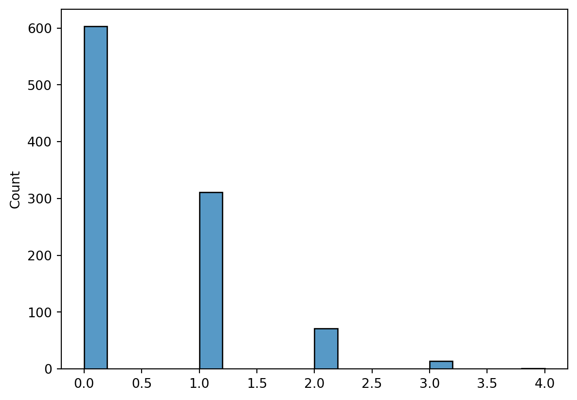
We have already encountered the Bernoulli distribution in the introduction to probability mass functions. The Bernoulli distribution is a discrete distribution with two possible outcomes, usually labeled 0 (failure) and 1 (success). The probability mass function of a Bernoulli distribution is given by:
f(x) = \begin{cases} p & \text{if } x = 1 \\ 1 - p & \text{if } x = 0 \end{cases}
and we have already computed its expected value and variance. Let X \sim \text{Binom}(1, p):
\begin{align*} E(X) & = p \\ \text{Var}(X) & = p(1-p) \end{align*}
The binomial distribution is a discrete distribution that models the number of successes in a fixed number of independent Bernoulli trials. Let X \sim \text{Binom}(n, p), where n \in \mathbb{N} is the number of trials and p > 0 is the probability of success in each trial. The probability mass function of a binomial distribution is given by:
f(x) = \binom{n}{x} p^x (1-p)^{n-x}, x = 0, 1, \ldots, n
where \binom{n}{x} is the binomial coefficient, which is the number of ways to choose x successes from n trials. The expected value and variance of a binomial distribution are:
A useful property of the binomial distribution is that it can be expressed as a sum of independent Bernoulli random variables. Let X_1, X_2, \ldots, X_n be independent Bernoulli random variables with parameter p. Then the sum X = X_1 + X_2 + \ldots + X_n follows a binomial distribution with parameters n and p.
Because the binomial distribution is a sum of independent Bernoulli random variables, we can use the linearity of expectation to compute its expected value and variance:
\begin{align*} E(X) & = E(X_1 + X_2 + \ldots + X_n) = E(X_1) + E(X_2) + \ldots + E(X_n) = np \\ \text{Var}(X) & = \text{Var}(X_1 + X_2 + \ldots + X_n) = \text{Var}(X_1) + \text{Var}(X_2) + \ldots + \text{Var}(X_n) = np(1-p) \end{align*}
The geometric distribution is a discrete distribution that models the number of trials needed to achieve the first success in a sequence of independent Bernoulli trials. Let X \sim \text{Geom}(p), where p > 0 is the probability of success in each trial. The probability mass function of a geometric distribution is given by:
f(x) = (1-p)^{x-1} p, x = 1, 2, \ldots
The expected value and variance of a geometric distribution are:
\begin{align*} E(X) & = \frac{1}{p} \\ \text{Var}(X) & = \frac{1-p}{p^2} \end{align*}
The Poisson distribution is a discrete distribution that models the number of events occurring in a fixed interval of time or space. Let X \sim \text{Poisson}(\lambda), where \lambda > 0 is the average rate of events. The probability mass function of a Poisson distribution is given by:
f(x) = \frac{e^{-\lambda} \lambda^x}{x!}, x = 0, 1, 2, \ldots
The expected value and variance of a Poisson distribution are:
\begin{align*} E(X) & = \lambda \\ \text{Var}(X) & = \lambda \end{align*}
# Select 1000 draws from a binomial distribution with p = 0.2 and n = 100
import numpy as np
import seaborn as sns
R = 1000
r02 = np.random.binomial(10, 0.05, R)
r02
sns.histplot(r02)
The negative binomial distribution is a discrete distribution that models the number of trials needed to achieve a fixed number of successes in a sequence of independent Bernoulli trials. Let X \sim \text{NegBinom}(r, p), where r \in \mathbb{N} is the number of successes and p > 0 is the probability of success in each trial. The probability mass function of a negative binomial distribution is given by:
f(x) = \binom{x-1}{r-1} p^r (1-p)^{x-r}, x = r, r+1, \ldots
The logic behind the the formula for the PMF of the negative binomial distribution is that we need to have r-1 successes in the first x-1 trials, and the x-th trial must be a success. As in the case of the binomial distribution, we can count the number of ordered sequences of successes and failures that satisfy these conditions and then divide their number by the number of permutations of the r - 1 successes and x - r failures before the last success. The total number of ordered sequences of size x - 1 with distinct elements is (x - 1)!. For the purpose of counting the number of successes, the r - 1 successes are indistinguishable, so we need to divide by (r - 1)!. Similarly, the x - r failures are indistinguishable, so we need to divide by (x - r)!. The number of ordered sequences of successes and failures that satisfy the conditions is then:
\frac{(x - 1)!}{(r - 1)!(x - r)!} = \binom{x-1}{r-1}
Each of these sequences has probability p^r (1-p)^{x-r} (including the last success) because we assume that the probability of success in each trial is p and therefore the probability of failure is 1 - p.
Exercise 11.1 (Another Birthday Problem) You are sitting in a room with 1000 people. Assume that each person has a birthday that is uniformly distributed over the 365 days of the year and that the birthdays are independent (disregard the 29th of February for simplicity). Let X be the number of people in the room that share a birthday with you. Write down the PMF of X and compute the probability of sharing a birthday with exactly one other person.
Exercise 11.2 (Call Center Availability) You are managing a small call center with 5 operators who work at any given time and are servicing 100,000 customers. Assume that each customer has a 0.005 percent chance of calling the call center at any given time (independently from the other customers). Let X be the number of customers who call the call center in the next hour. What is the probability that all 5 operators are busy?
Exercise 11.3 (Number of Calls until Connection) Let’s continue the call center example. Assume that a customer has a 20 percent probability of reaching an operator when calling the call center. Let X be the number of calls a customer makes until they reach an operator.
Exercise 11.4 Suppose that the number of customers arriving at a store follows a Poisson distribution with an average rate of 5 customers per hour. What is the probability that exactly 3 customers arrive in a given hour?