Until now we have been dealing with discrete distributions, where the random variable can only take on a finite number of values. In this notebook, we will introduce continuous distributions, where the random variable can take on any value in a given range.
The continuous distributions differ from the discrete distributions in that the probability of a single value is zero. Instead, the probability is defined over intervals. Just like the probability mass function fully describes a discrete distribution, a continuous distribution is fully described by its probability density function (PDF).
A PDF is a non-negative function f(x) that integrates to 1 over the entire real line. Let X be a continuous random variable with PDF f(x). Then, for any two values.
P(a \leq X \leq b) = \int_{a}^{b} f(x) dx
The CDF of a continuous random variable is defined just as in the discrete case with the sum replaced by an integral:
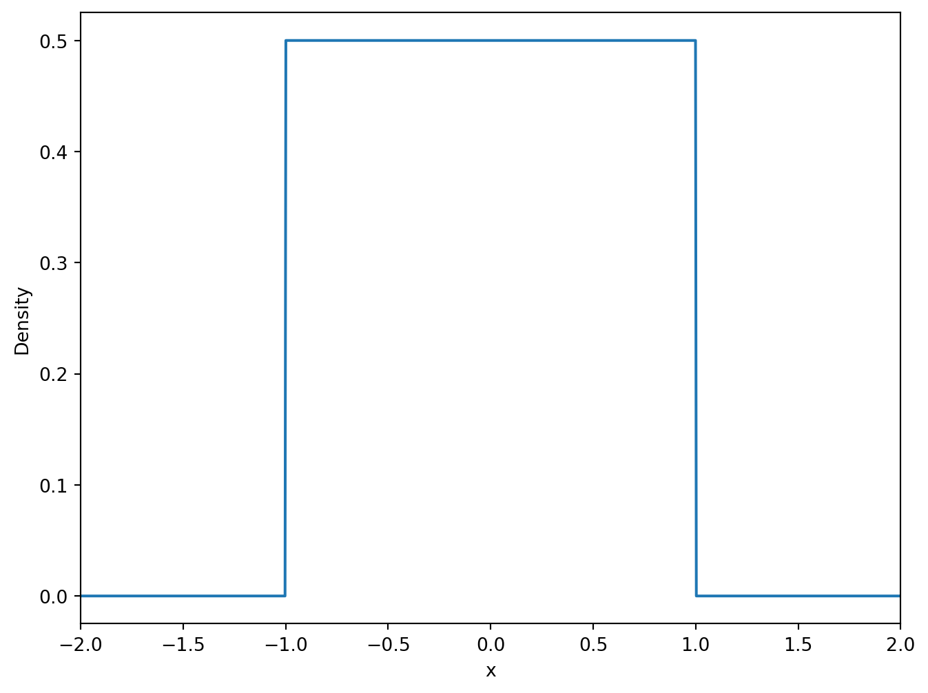
The density function of the uniform distribution is a constant over the interval ([-1, 1]). The probability of the random variable falling in any subinterval of ([-1, 1]) is proportional to the length of the subinterval.
import matplotlib.pyplot as pltimport numpy as npimport pandas as pdimport seaborn as snsfrom scipy import stats# Define the range of xx = np.linspace(-2, 2, 1000)# Calculate the density of the uniform distributiony = stats.uniform.pdf(x, loc=-1, scale=2)# Create the plotplt.figure(figsize=(8, 6))plt.plot(x, y)plt.xlim([-2, 2])plt.xlabel('x')plt.ylabel('Density')
Text(0, 0.5, 'Density')
# Draw 10 random values from the uniform distribution between -1 and 1x_unif = np.random.uniform(low=-1, high=1, size=10)x_unif
# How many of the random numbers are smaller than 0? Use np.sum to count the number of random numbers that satisfy the condition.print("Number of results less than zero =", np.sum(x_unif <0))# How many of the random numbers are between 0 and 0.5?print("Number of results between 0 and 0.5 =", np.sum((x_unif >0) & (x_unif <0.5)))
Number of results less than zero = 3
Number of results between 0 and 0.5 = 3
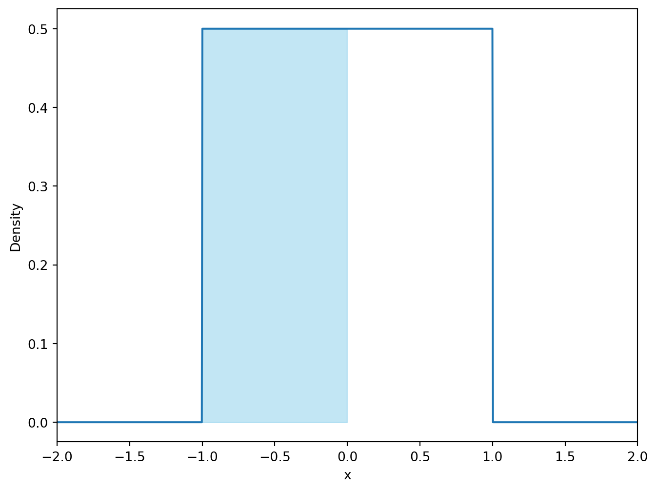
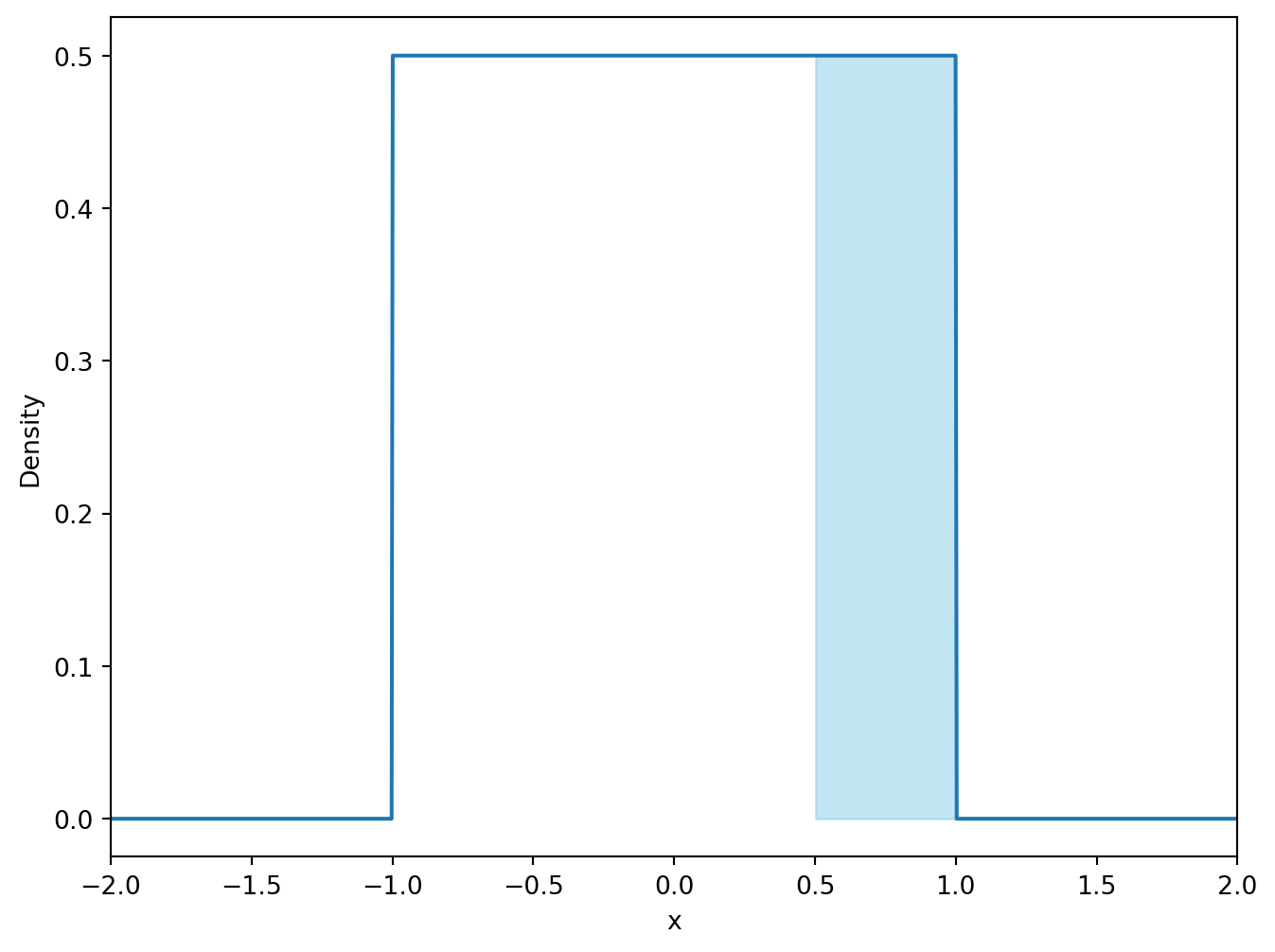
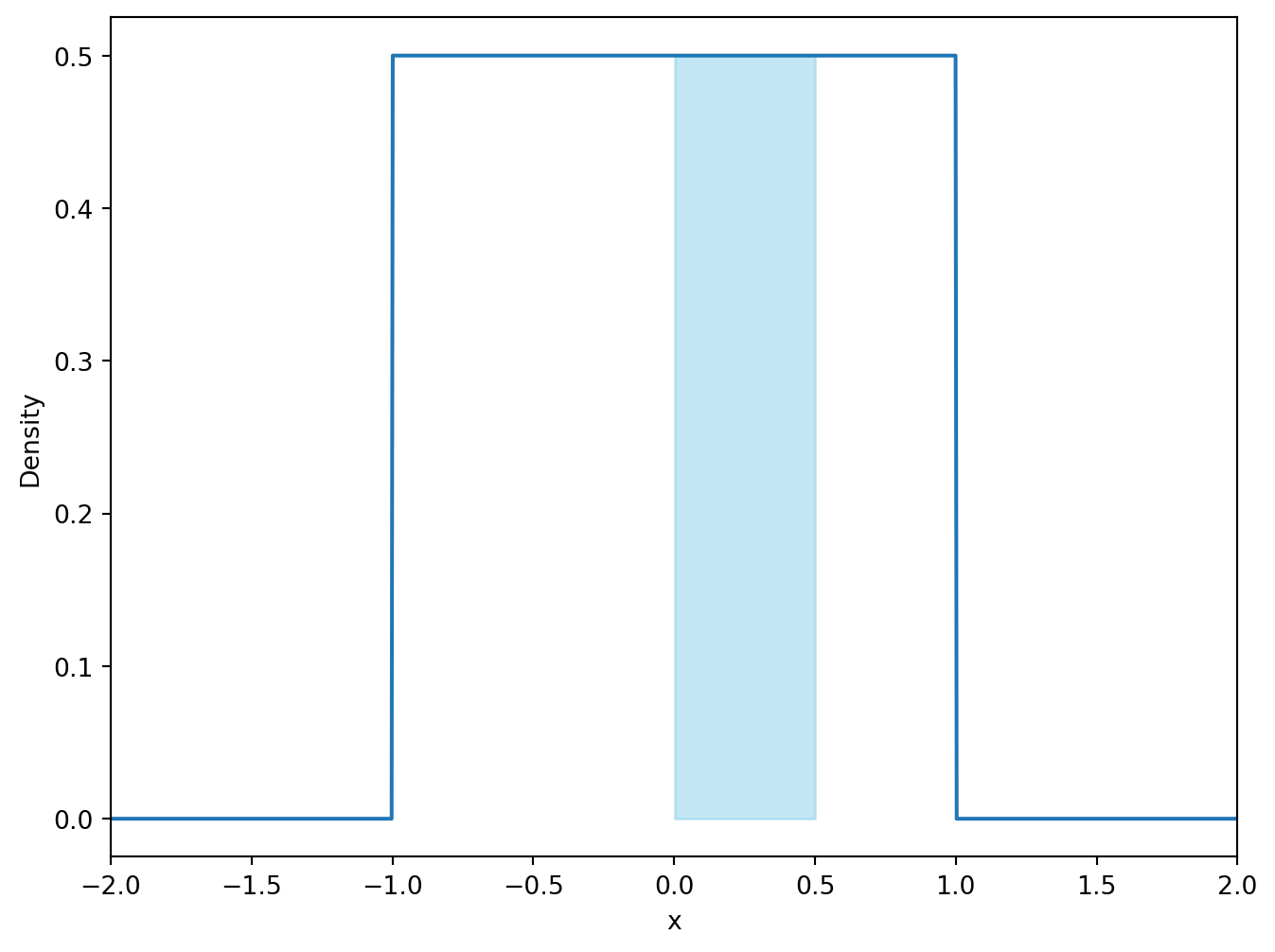
# Calculate the probability of X being less than 0. (https://docs.scipy.org/doc/scipy/reference/generated/scipy.stats.uniform.html)print("P(X < 0) =", stats.uniform.cdf(0, loc=-1, scale=2))# Calculate the probability of X being greater than 0.5.print("P(X > 0.5) =", 1- stats.uniform.cdf(0.5, loc=-1, scale=2))# Calculate the probability that the event X is in the interval [0, 0.5] occurs.print("P(0 < X < 0.5) =", stats.uniform.cdf(0.5, loc=-1, scale=2) - stats.uniform.cdf(0, loc=-1, scale=2))# Compare the probability with the number of values in the simulation that lie in the interval [0, 0.5].print("Number of values in the interval [0, 0.5]:", np.sum((x_unif >0) & (x_unif <0.5)))print("Share of values in the interval [0, 0.5]:", np.mean((x_unif >0) & (x_unif <0.5)))
P(X < 0) = 0.5
P(X > 0.5) = 0.25
P(0 < X < 0.5) = 0.25
Number of values in the interval [0, 0.5]: 3
Share of values in the interval [0, 0.5]: 0.3
# Visualize the probability of X being less than 0 as the area under the curve.plt.figure(figsize=(8, 6))plt.plot(x, y)plt.fill_between(x, y, where=(x <0), color='skyblue', alpha=0.5)plt.xlim([-2, 2])plt.xlabel('x')plt.ylabel('Density')
Text(0, 0.5, 'Density')
# Visualize the probability of X being greater than 0.5 as the area under the curve.plt.figure(figsize=(8, 6))plt.plot(x, y)plt.fill_between(x, y, where=(x >0.5), color='skyblue', alpha=0.5)plt.xlim([-2, 2])plt.xlabel('x')plt.ylabel('Density')
Text(0, 0.5, 'Density')
# Visualize the probability of X being in the interval [0, 0.5] as the area under the curve.plt.figure(figsize=(8, 6))plt.plot(x, y)plt.fill_between(x, y, where=((x >0) & (x <0.5)), color='skyblue', alpha=0.5)plt.xlim([-2, 2])plt.xlabel('x')plt.ylabel('Density')
Text(0, 0.5, 'Density')
12.2 Moments of a Continuous Distribution
The moments of a continuous distribution are defined in the same way as for a discrete distribution, but the summation is replaced by an integral. The expected value of a continuous random variable X is given by:
E(X) = \int_{-\infty}^{\infty} x f(x) dx
The variance of a continuous random variable X is given by:
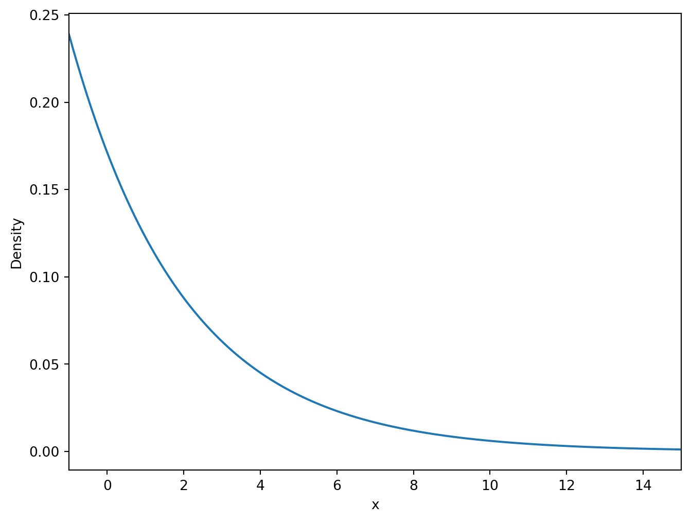
We have already seen the geometric distribution, which models the number of trials until the first success in a sequence of independent Bernoulli trials. The exponential distribution is the continuous analog of the geometric distribution.
The PDF of the exponential distribution is given by:
f(x) = \begin{cases}
\lambda e^{-\lambda x} & x \geq 0\\
0 & x < 0
\end{cases}
Exercise 13.1 (CDF of the Exponential Distribution) Calculate the CDF of the exponential distribution.
Solution (click to expand)
The CDF of the exponential distribution is given by:
Exercise 13.2 (Expected Value of the Exponential Distribution) Calculate the expected value of the exponential distribution.
Solution (click to expand)
To calculate the expected value of the exponential distribution, we need to evaluate the following integral:
\begin{align*}
E(X) & = \int_{-\infty}^{\infty} x \lambda e^{-\lambda x} dx = \int_{0}^{\infty} x \lambda e^{-\lambda x} dx
\end{align*}
We can use integration by parts to solve this integral. The integration by parts rule is related to the product rule for differentiation.
(uv)' = u'v + uv'
where both u and v are functions of x and u' and v' are their derivatives with respect to x. Integrate both sides and rearrange to get the integration by parts formula:
In our integral it makes sense to choose u = \lambda x and v' = e^{-\lambda x} because the derivative of u is a constant and the integral of v' is easy to calculate. Note that
\int e^{-\lambda x} = \frac{e^{-\lambda x}}{-\lambda} + C
where C is the constant of integration. Now we are ready to apply the integration by parts formula:
Note that the last result uses the fact that \lim_{x \to \infty} e^{-\lambda x} = 0 and \lim_{x \to \infty} x e^{-\lambda x} = 0. The latter limit can be shown by applying L’Hopital’s rule.
To find the variance of the exponential distribution, we can find the second uncentered momen of the distribution (i.e., E(X^2)) and then use the formula \text{Var}(X) = E(X^2) - E(X)^2. Again, we can use integration by parts to find the integral.
# Create a grid of 1000 points between -1 and 15x = np.linspace(-1, 15, 1000)# Calculate the density of the exponential distribution with rate parameter 1y = stats.expon.pdf(x, loc=-2, scale=3)# Create the plotplt.figure(figsize=(8, 6))plt.plot(x, y)plt.xlim([-1, 15])plt.xlabel('x')plt.ylabel('Density')
Text(0, 0.5, 'Density')
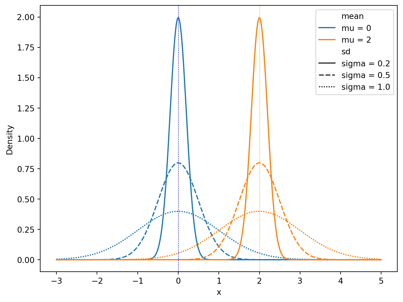
13.1 The Normal Distribution
The normal distribution is the most important continuous distribution in statistics. It is symmetric around the mean and has a bell-shaped curve. The PDF of the normal distribution is given by:
to say that X is normally distributed with mean \mu and variance \sigma^2. You do not need to memorize the formula for the normal distribution PDF, but you should a couple of important properties:
# Visualize the density of the normal distribution with different means and standard deviations# Define the means and standard deviations for which we want to plot the normal distributionmeans = [0, 2]sds = [0.2, 0.5, 1]# Create a grid of x valuesx = np.linspace(-3, 5, 500)# Create a DataFrame with all combinations of means, sds, and x valuesdf = pd.DataFrame([(mean, sd, x_val, stats.norm.pdf(x_val, mean, sd)) for mean in means for sd in sds for x_val in x], columns=['mean', 'sd', 'x', 'y'])# Create labels for mean and sddf['mean'] =r'mu = '+ df['mean'].astype(str)df['sd'] =r'sigma = '+ df['sd'].astype(str)# Plotplt.figure(figsize=(8, 6))sns.lineplot(data=df, x='x', y='y', hue='mean', style='sd')plt.axvline(0, color='blue', linestyle='--', linewidth=0.5)plt.axvline(2, color='orange', linestyle='--', linewidth=0.5)plt.xlabel('x')plt.ylabel('Density')
If X \sim N(\mu, \sigma^2), then Z = \frac{X - \mu}{\sigma} \sim N(0, 1) is called the standard normal distribution. The standard normal distribution has mean 0 and variance 1.
If X_1, X_2, \ldots, X_n are independent and identically distributed (i.i.d.) random variables with mean \mu and variance \sigma^2, then sum of the random variables is normally distributed:
\sum_{i=1}^{n} X_i \sim N(n\mu, n\sigma^2)
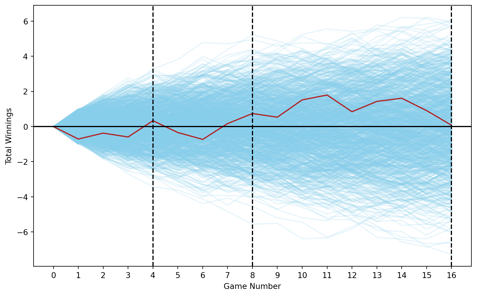
It turns out the sum of independent random variables from any distribution (as long as the variance is finite) approaches a normal distribution as the number of variables increases. This is known as the central limit theorem. The central limit theorem is one of the most important results in statistics and is the reason why the normal distribution is so important.
Theorem 13.1 (Central Limit Theorem) Let X_1, X_2, \ldots, X_n be i.i.d. random variables with mean \mu and variance \sigma^2. Let S_n = \sum_{i=1}^{n} X_i. Then, as n approaches infinity, the distribution of \frac{S_n - n\mu}{\sqrt{n}\sigma} approaches the standard normal distribution.
players_n =1000games_n =16# Create a DataFrame similar to expand_grid in Runif_games = pd.DataFrame( np.array( np.meshgrid( np.arange(1, games_n +1), np.arange(1, players_n +1) )).T.reshape(-1, 2), columns=['game', 'player'])# Add result column with random uniform values between -1 and 1unif_games['result'] = np.random.uniform(-1, 1, size=len(unif_games))# Add initial values for each playerinitial_values = pd.DataFrame( {'player': np.arange(1, players_n +1), 'game': 0, 'result': 0})unif_games = pd.concat([unif_games, initial_values])# Sort values and calculate running total for each playerunif_games = unif_games.sort_values(['player', 'game'])unif_games['running_total'] = unif_games.groupby('player')['result'].cumsum()# Plottingplt.figure(figsize=(10, 6))for player in unif_games['player'].unique(): player_data = unif_games[unif_games['player'] == player] plt.plot(player_data['game'], player_data['running_total'], color='skyblue', alpha=0.2)# First playerplayer_data = unif_games[unif_games['player'] ==1]plt.plot(player_data['game'], player_data['running_total'], color='firebrick', label='Player 1')plt.axhline(0, color='black')for mark in [4, 8, 16]: plt.axvline(x=mark, linestyle='--', color='black')plt.xlabel('Game Number')plt.ylabel('Total Winnings')plt.xticks(range(0, 17, 1))
([<matplotlib.axis.XTick at 0x7f33a013ab10>,
  <matplotlib.axis.XTick at 0x7f33a01520c0>,
  <matplotlib.axis.XTick at 0x7f339f543d10>,
  <matplotlib.axis.XTick at 0x7f339f40ffe0>,
  <matplotlib.axis.XTick at 0x7f339f3b12b0>,
  <matplotlib.axis.XTick at 0x7f339fc9b1a0>,
  <matplotlib.axis.XTick at 0x7f339f3b1c70>,
  <matplotlib.axis.XTick at 0x7f339f3b24e0>,
  <matplotlib.axis.XTick at 0x7f339f3b2d50>,
  <matplotlib.axis.XTick at 0x7f339f3b3650>,
  <matplotlib.axis.XTick at 0x7f339ff85160>,
  <matplotlib.axis.XTick at 0x7f339f3b26c0>,
  <matplotlib.axis.XTick at 0x7f339f3e43b0>,
  <matplotlib.axis.XTick at 0x7f339f3e4c50>,
  <matplotlib.axis.XTick at 0x7f339f3e55e0>,
  <matplotlib.axis.XTick at 0x7f339f3e5d30>,
  <matplotlib.axis.XTick at 0x7f339f3b31d0>],
 [Text(0, 0, '0'),
  Text(1, 0, '1'),
  Text(2, 0, '2'),
  Text(3, 0, '3'),
  Text(4, 0, '4'),
  Text(5, 0, '5'),
  Text(6, 0, '6'),
  Text(7, 0, '7'),
  Text(8, 0, '8'),
  Text(9, 0, '9'),
  Text(10, 0, '10'),
  Text(11, 0, '11'),
  Text(12, 0, '12'),
  Text(13, 0, '13'),
  Text(14, 0, '14'),
  Text(15, 0, '15'),
  Text(16, 0, '16')])
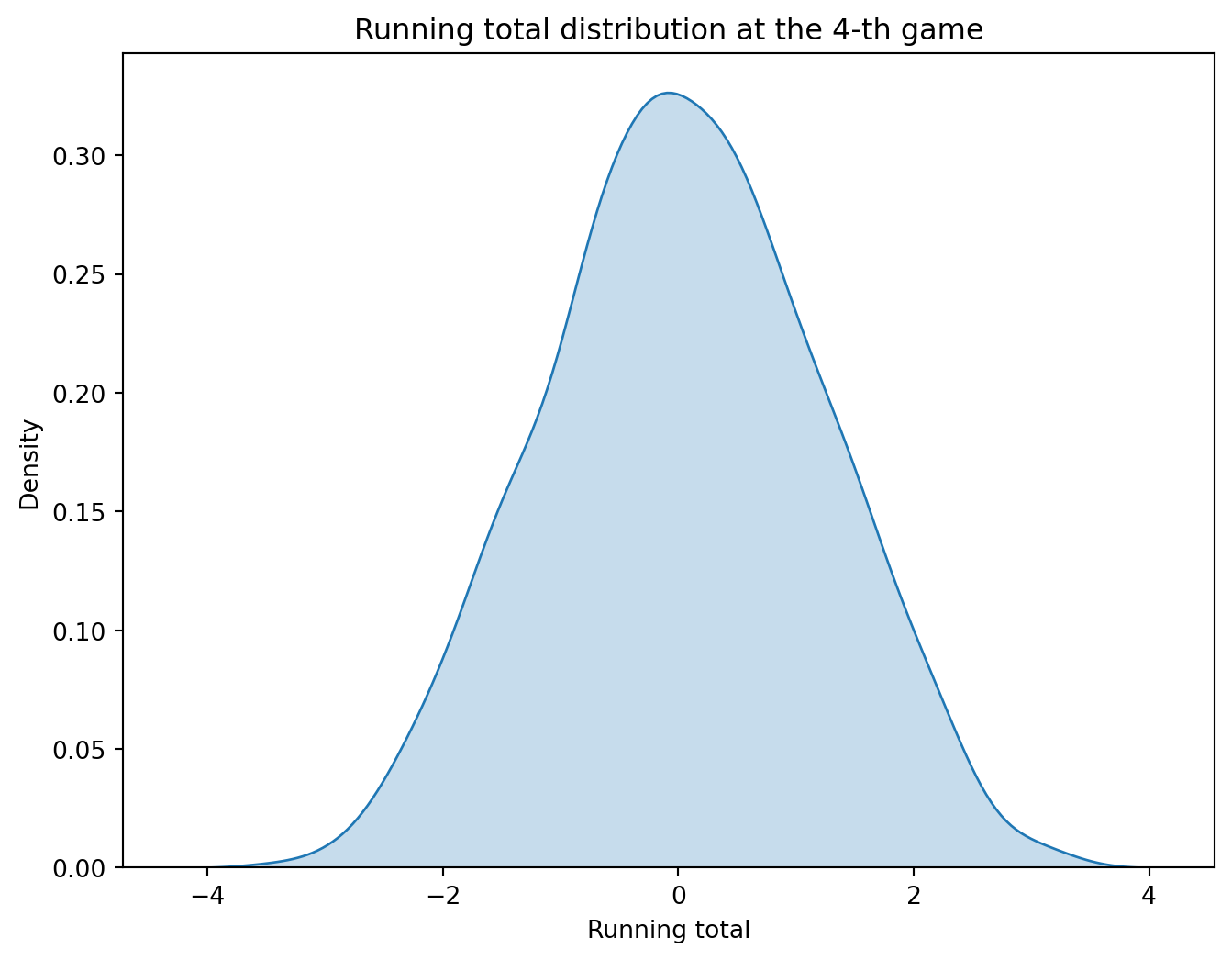
game_4 = unif_games[unif_games['game'] ==4]plt.figure(figsize=(8, 6))sns.kdeplot(data=game_4, x='running_total', fill=True)plt.title('Running total distribution at the 4-th game')plt.xlabel('Running total')
Text(0.5, 0, 'Running total')
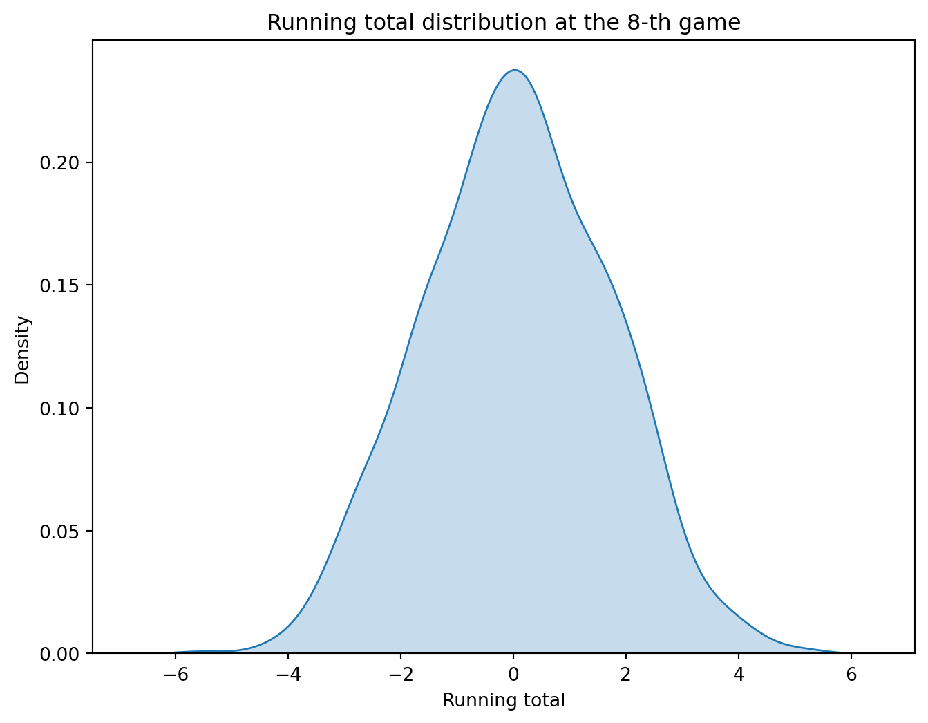
# Density estimate plot for the 8-th gamegame_8 = unif_games[unif_games['game'] ==8]plt.figure(figsize=(8, 6))sns.kdeplot(data=game_8, x='running_total', fill=True)plt.title('Running total distribution at the 8-th game')plt.xlabel('Running total')
Text(0.5, 0, 'Running total')
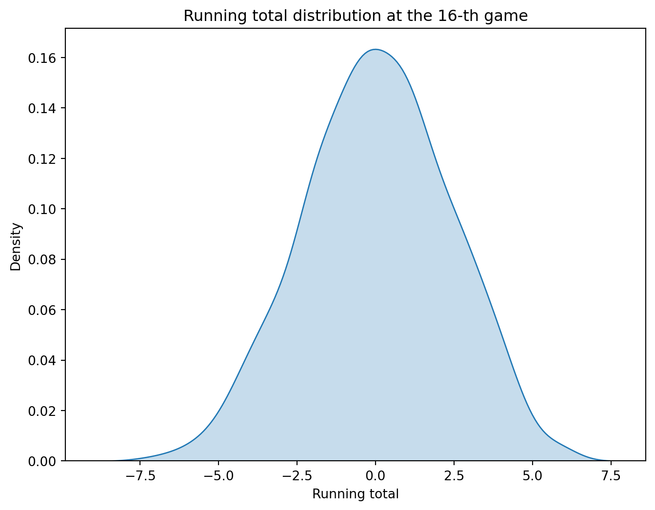
game_16 = unif_games[unif_games['game'] ==16]plt.figure(figsize=(8, 6))sns.kdeplot(data=game_16, x='running_total', fill=True)plt.title('Running total distribution at the 16-th game')plt.xlabel('Running total')
Text(0.5, 0, 'Running total')
13.2 Probabilities of the Normal Distribution
As with other distributions, we can calculate probabilities with the normal distribution using the CDF, which is the integral of the PDF over the interval (-, x). The CDF of the normal distribution does not have a closed-form solution, but it can be calculated using numerical methods or software. Before the advent of computers, tables were used to look up the values of the CDF for different values of (x). These tables are known as z-tables. As it is not possible to create tables for all possible values of () and (), the tables are usually for the standard normal distribution, so we need to standardize the random variable before looking up the value in the table.
13.3 Standardizing a Random Variable
For any random variable with expected value () and variance (^2), we can standardize the random variable by subtracting the mean and dividing by the standard deviation:
Z = \frac{X - \mu}{\sigma}
The resulting random variable (Z) has mean 0 and variance 1. To see this, simply calculate the expected value and variance of (Z):
Note that \mu and \sigma are not random variables but constants.
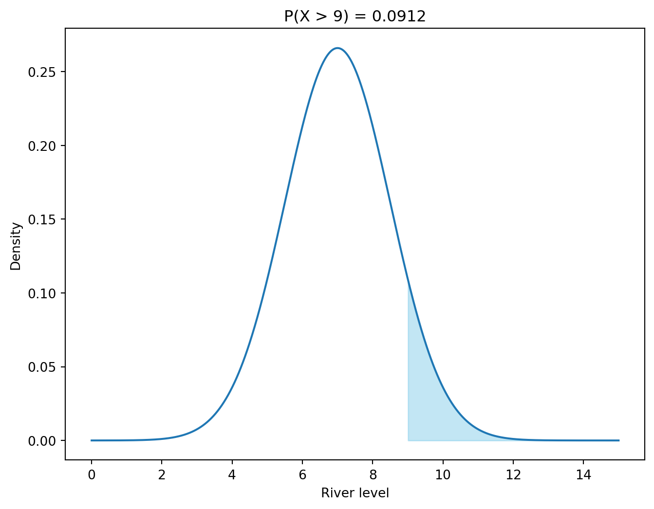
Exercise 13.3 (Probabilities with the Normal Distribution) Calculate the following probabilities for the standard normal distribution. Let the level of a river be normally distributed with mean 7 (meters) and standard deviation (\sigma) 1.5. Let us say that the river is in flood when the level is above 9 meters and in drought when the level is below 5 meters.
What is the probability that the river is in flood?
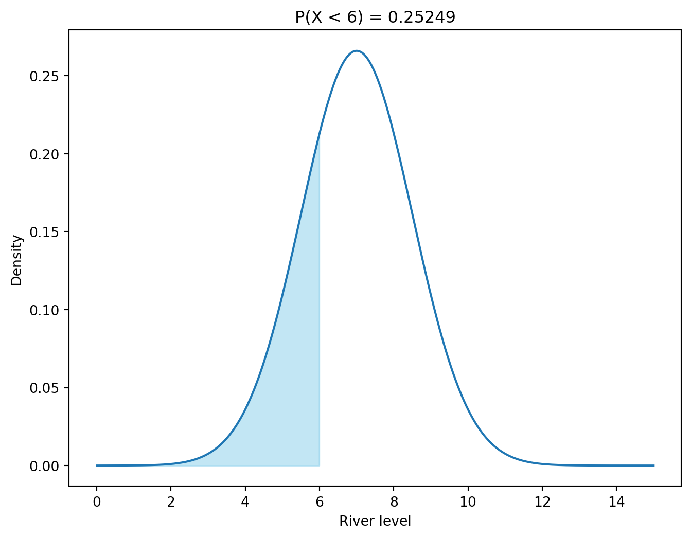
What is the probability that the river is in drought?
What is the probability that the river is between 5 and 9 meters?
Solution (click to expand)
The probability that the river is in flood is given by:
P(X > 9) = 1 - P(X \leq 9) = 1 - F(9)
where (F(x)) is the CDF of the normal distribution. With access to computer software, we can compute the CDF directly (see the result below). If you must use a z-table, you need to standardize first:
# Compute the probabilities with scipy.stats# Probability that the river level is over 9 meters. In the following code loc is the mean and scale is the standard deviation.print(1- stats.norm.cdf(9, loc=7, scale=1.5))# The same probability using the standard normal distributionprint(1- stats.norm.cdf((9-7) /1.5))
0.09121121972586788
0.09121121972586788
# Show the probability as an area under the curvex = np.linspace(0, 15, 1000)y = stats.norm.pdf(x, loc=7, scale=1.5)plt.figure(figsize=(8, 6))plt.plot(x, y)plt.fill_between(x, y, where=(x >9), color='skyblue', alpha=0.5)plt.xlabel('River level')plt.ylabel('Density')plt.title('P(X > 9) = 0.0912')
Text(0.5, 1.0, 'P(X > 9) = 0.0912')
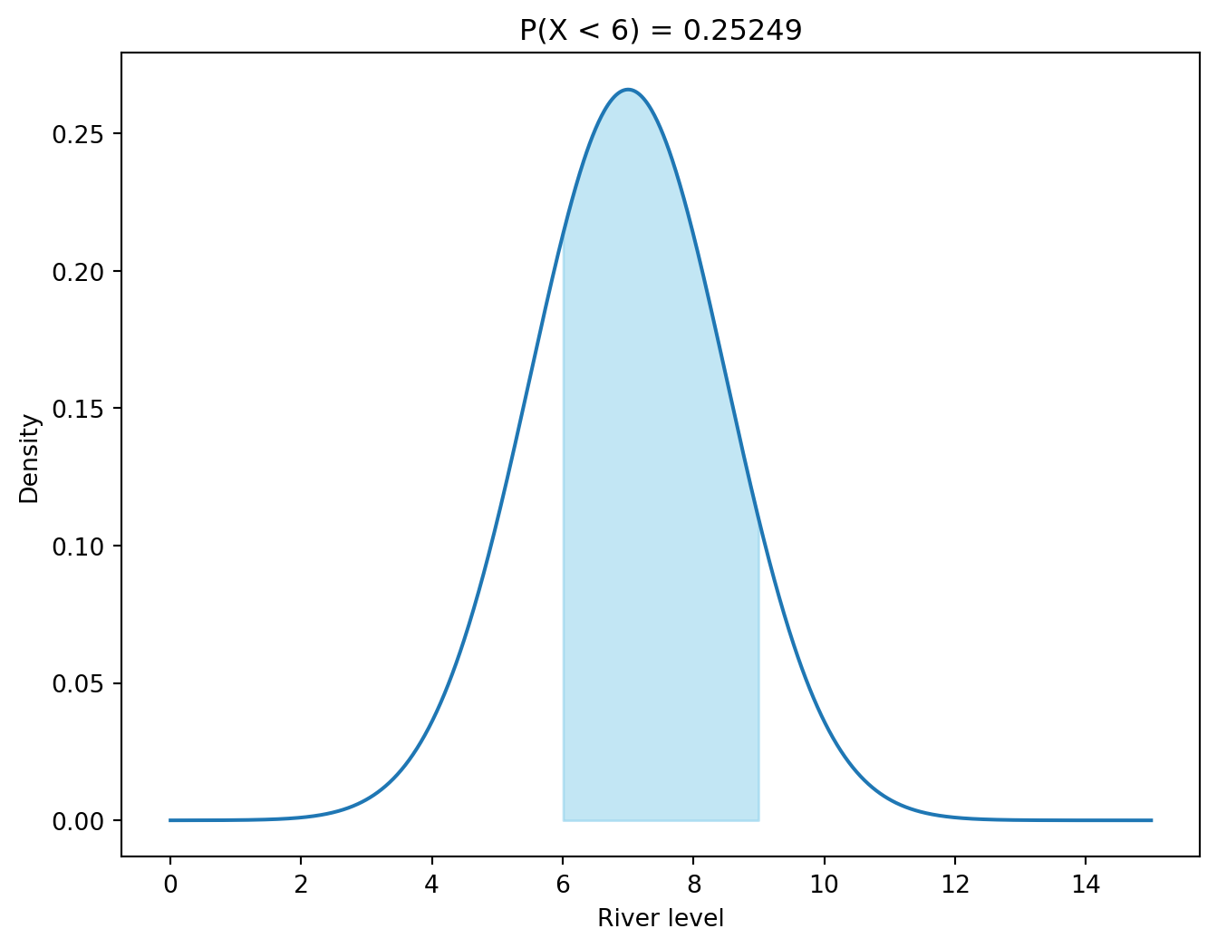
# Probability that the river is in drought (below 6 meters).print(stats.norm.cdf(6, loc=7, scale=1.5))# The same probability using the standard normal distribution.print(stats.norm.cdf((6-7) /1.5))
# Probability that the river level is between 6 and 9 meters (not in drought and not in flood)print(stats.norm.cdf(9, loc=7, scale=1.5) - stats.norm.cdf(6, loc=7, scale=1.5))# The same probability, calculated using the standard normal distributionprint(stats.norm.cdf((9-7) /1.5) - stats.norm.cdf((6-7) /1.5))
# Create a z-table for the import pandas as pdimport numpy as npfrom scipy.stats import norm# Define the range of z-scoresz_scores = np.arange(-3.0, 3.1, 0.1)# Calculate the probabilities for each z-scoreprobabilities = norm.cdf(z_scores)# Create a DataFramedf = pd.DataFrame({'z': z_scores,'P(x < Z)': probabilities})df
z
P(x < Z)
0
-3.0
0.001350
1
-2.9
0.001866
2
-2.8
0.002555
3
-2.7
0.003467
4
-2.6
0.004661
...
...
...
56
2.6
0.995339
57
2.7
0.996533
58
2.8
0.997445
59
2.9
0.998134
60
3.0
0.998650
61 rows × 2 columns
Exercise 13.4 Assume that the weight of adults in Sofia is normally distributed with mean 70 kg and standard deviation 10 kg. The lift in a building can carry a maximum of 550 kg. What is the probability that carry capacity of the lift is exceeded if 7 adults enter the lift?
Solution (click to expand)
# Calculate the probability
# Sample 5 persons at random from a normal population with mean 70 and sd = 10import numpy as npR =100000n =7mu =70sd =10simulations = np.random.randn(R, n)*10+70simulations
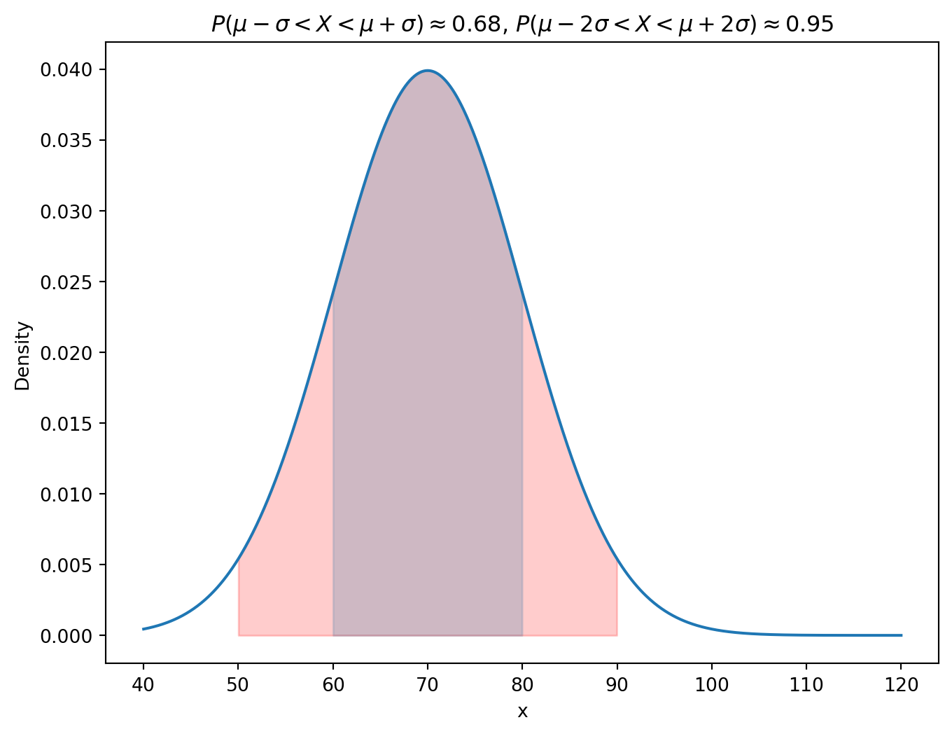
For a normal distribution, the probability that a random variable falls within a certain number of standard deviations from the mean can be calculated using the CDF. The probability that a random variable falls within one standard deviation of the mean is approximately 68%, within two standard deviations is approximately 95%, and within three standard deviations is approximately 99.7%.
Let X \sim N(\mu, \sigma^2):
P(\mu - \sigma < X < \mu + \sigma) \approx 0.68
P(\mu - 2\sigma < X < \mu + 2\sigma) \approx 0.95
P(\mu - 3\sigma < X < \mu + 3\sigma) \approx 0.99
# See this with code# Run the code for different value of mu and sd and see that the probabilities don't changemu =70sd =10# One sigma above and below the meanprint(stats.norm.cdf(mu + sd, loc=mu, scale=sd) - stats.norm.cdf(mu - sd, loc=mu, scale=sd))# Two sigma above and below the meanprint(stats.norm.cdf(mu +2*sd, loc=mu, scale=sd) - stats.norm.cdf(mu -2*sd, loc=mu, scale=sd))# Three sigma above and below the meanprint(stats.norm.cdf(mu +3*sd, loc=mu, scale=sd) - stats.norm.cdf(mu -3*sd, loc=mu, scale=sd))
# Visualize the probability for one sigma above and below the meanx = np.linspace(40, 120, 1000)y = stats.norm.pdf(x, loc=mu, scale=sd)plt.figure(figsize=(8, 6))plt.plot(x, y)plt.fill_between(x, y, where=((x > mu - sd) & (x < mu + sd)), color='skyblue', alpha=0.5)plt.fill_between(x, y, where=((x > mu -2*sd) & (x < mu +2* sd)), color='red', alpha=0.2)plt.xlabel('x')plt.ylabel('Density')plt.title(r'$P(\mu - \sigma < X < \mu + \sigma) \approx 0.68$, $P(\mu - 2\sigma < X < \mu + 2\sigma) \approx 0.95$')
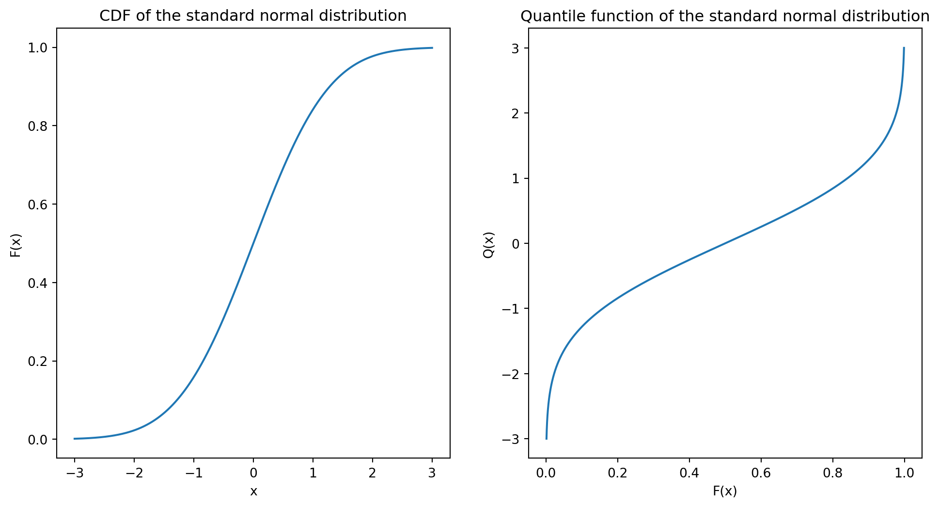
The CDF of a random variable gives the probability that the random variable is less than or equal to a given value. The quantile function is the inverse of the CDF and gives the value of the random variable for a given probability. For example, the 0.95 quantile of a random variable is the value such that the probability of the random variable being less than or equal to that value is 0.95. As there is no closed-form solution for the CDF of the normal distribution, you will need to use numerical methods (implemented in software) to calculate the quantile function or use tables.
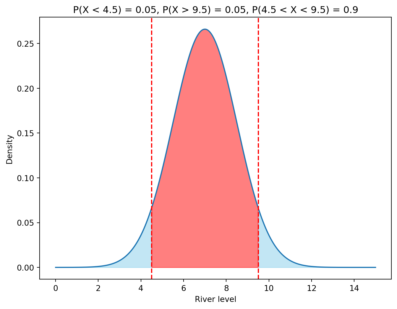
Exercise 13.5 (River Level Quantiles)
Let us continue the example with the river level. What is the level of the river such that the probability of the river being below that level is 0.05 (the 0.05 quantile)?
What is the level of the river such that the probability of the river being above that level is 0.05 (the 0.95 quantile)?
# Plot the CFD and the quantile function for the standard normal distribution# Create a grid of x valuesx = np.linspace(-3, 3, 1000)# Calculate the CDF of the standard normal distributiony_cdf = stats.norm.cdf(x)# Calculate the quantile function of the standard normal distributiony_quantile = stats.norm.ppf(y_cdf)# Create the plotplt.figure(figsize=(12, 6))plt.subplot(1, 2, 1)plt.plot(x, y_cdf)plt.xlabel('x')plt.ylabel('F(x)')plt.title('CDF of the standard normal distribution')plt.subplot(1, 2, 2)plt.plot(y_cdf, x)plt.xlabel('F(x)')plt.ylabel('Q(x)')plt.title('Quantile function of the standard normal distribution')
Text(0.5, 1.0, 'Quantile function of the standard normal distribution')
# Calculate the 0.05 quantile using the quantile function (called ppf (percentage point function) in scipy.stats)print(stats.norm.ppf(0.05, loc=7, scale=1.5))print(stats.norm.ppf(0.95, loc=7, scale=1.5))
4.532719559572791
9.467280440427208
# Visualize the quantiles on the density plotx = np.linspace(0, 15, 1000)y = stats.norm.pdf(x, loc=7, scale=1.5)plt.figure(figsize=(8, 6))plt.plot(x, y)plt.fill_between(x, y, where=(x <4.5), color='skyblue', alpha=0.5)plt.fill_between(x, y, where=(x >9.5), color='skyblue', alpha=0.5)plt.fill_between(x, y, where=(x >4.5) & (x <9.5), color='red', alpha=0.5)plt.axvline(4.5, color='red', linestyle='--')plt.axvline(9.5, color='red', linestyle='--')plt.xlabel('River level')plt.ylabel('Density')plt.title('P(X < 4.5) = 0.05, P(X > 9.5) = 0.05, P(4.5 < X < 9.5) = 0.9')
If you must use a z-table for the quantiles, you need to standardize first, because these tables usually only list the quantiles for the standard normal distribution.
# Create a z-table for the quantiles of the standard normal distributionimport pandas as pdimport numpy as np# Define the range of probabilitiesprobabilities = np.arange(0.0, 0.11, 0.01)# Calculate the quantiles for each probabilityquantiles = stats.norm.ppf(probabilities)# Create a DataFramedf = pd.DataFrame({'P(x < Z)': probabilities,'Q(p)': quantiles})df
P(x < Z)
Q(p)
0
0.00
-inf
1
0.01
-2.326348
2
0.02
-2.053749
3
0.03
-1.880794
4
0.04
-1.750686
5
0.05
-1.644854
6
0.06
-1.554774
7
0.07
-1.475791
8
0.08
-1.405072
9
0.09
-1.340755
10
0.10
-1.281552
# To find the 0.05 quantile of the normal distribution with mean 7 and standard deviation 1.5 using a z-table# we can first find the corresponding quantile of the standard normal distribution and then transform it back to the original scale.# Find the 0.05 quantile of the standard normal distribution z = stats.norm.ppf(0.05) # You can also look it up in the table abovez# Transform the quantile back to the original scalequantile =7+1.5* zquantile
4.532719559572791
# Check the result using the quantile function of the normal distribution with mean 7 and standard deviation 1.5stats.norm.ppf(0.05, loc=7, scale=1.5)